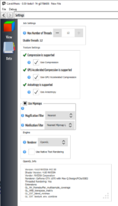
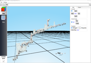
Out of the box, CaveWhere runs on a variety of platforms and computers. CaveWhere is implemented with OpenGL, a widely available and well supported graphics standard. Since OpenGL is a standard, it must be implemented by specific graphics vendors (such as NVidia, AMD, or Intel). Each vendors implementation of specific OpenGL extensions varies slightly. CaveWhere tries to detect the best possible rendering settings and use those settings to give you high performance rendering of your cave maps. This article tries to demystify the settings, shown below, to allow you to optimize CaveWhere for your computer.

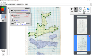
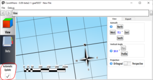
Going to File->Settings (on Windows and Linux) or (CaveWhere -> Preferences) on MacOS, the Settings Page will appear. On this page, there is several rendering options, to play around with. Most of these options CaveWhere will apply them immediately, but a few require you to restart CaveWhere.
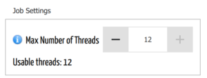
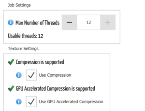
Job Settings
Job Settings allows you control the number of concurrent jobs that CaveWhere uses with a maximun number of threads. If you have a computer that’s less than 15 years old, it probably has multiple processing cores. You can see the number of available threads on your system described as “Usable threads:.” The system in the screenshot above has 12 available threads, meaning CaveWhere can do 12 jobs at the same time. By default, CaveWhere uses as many threads that exist on the system, giving you the best possible performance. If your computer overheats easily or you want to limit CaveWhere’s access to processing resources, you can reduce the access to the number of threads.
Texture Settings
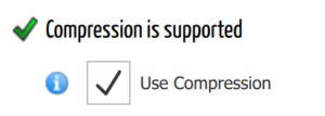
Texture Compression Support
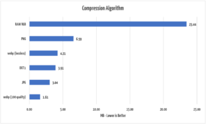
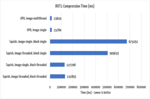
By default, CaveWhere uses DXT1 texture compression, unless it is not supported. DXT1 texture compression reduces the amount of video memory and allows you to visualize six times more cave. Check out the Compress article for details.
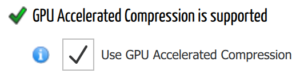
GPU Texture Compression Support
If your computer supports GPU Accelerated Compression, CaveWhere, by default, will use your GPU to compress textures. Turning this off will use a CPU implementation, which is slower, but higher quality than the GPU implementation. For more details, checkout the Compression article.
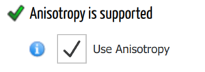
Anisotropy Support
If your graphics card supports Anisotropy, it is enabled by default. Anisotropy texture rendering improves the rendering quality by filtering textures and, overall, reduces rendering artifacts. It reduces rendering performance but should not be noticeable with most graphics cards. The illunstrations below show the difference between using Anisotropy and disabling it.
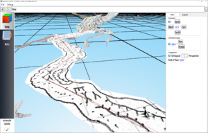
Anisotropy Enabled
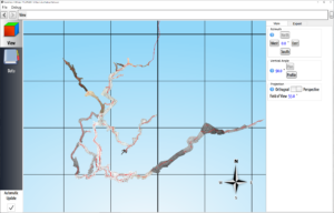
Disabled Anisotropy
The differences are subtle and are more noticeable in CaveWhere compared to these screenshots. Anisotropy produces better rendering results by using mipmaps.
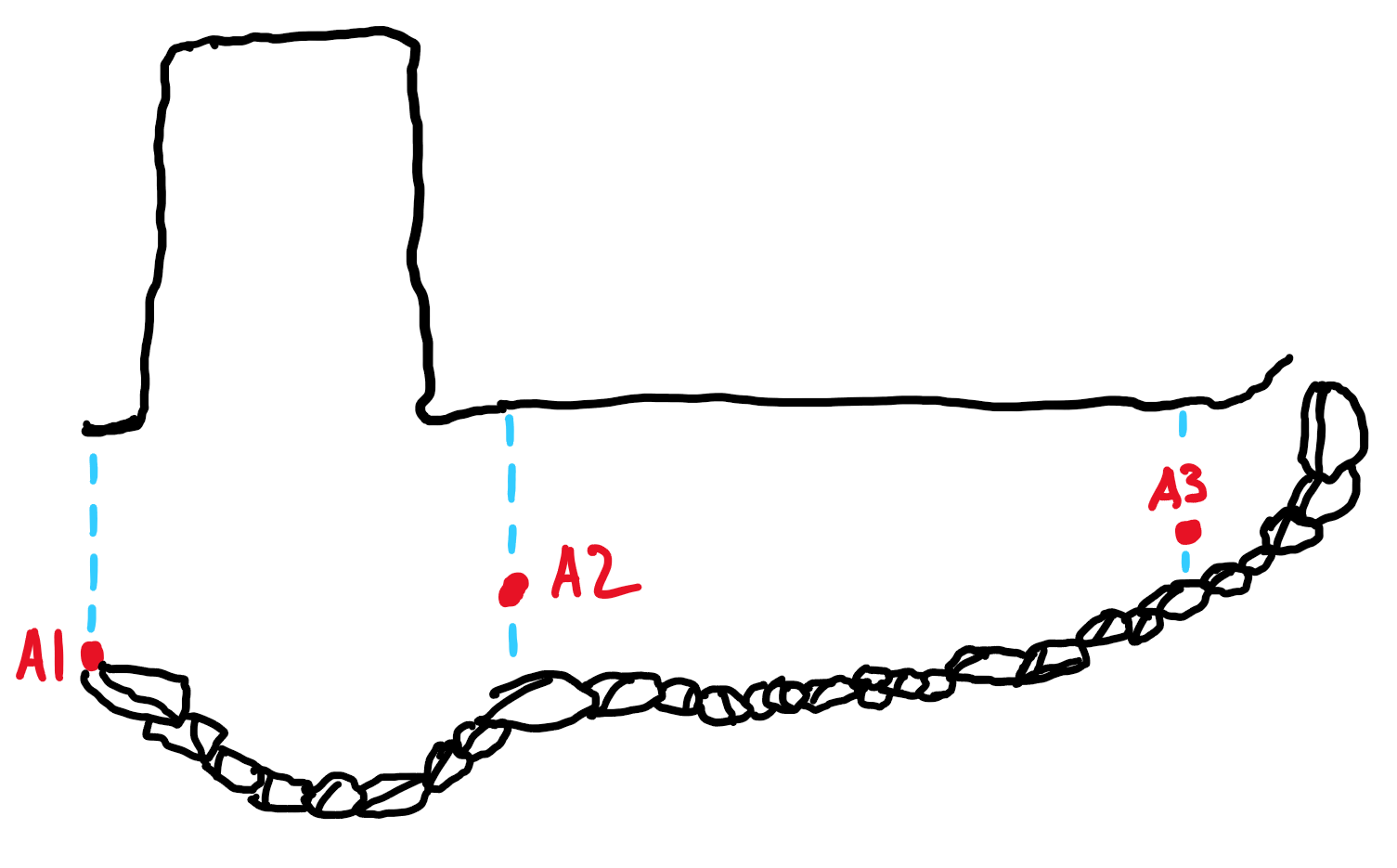
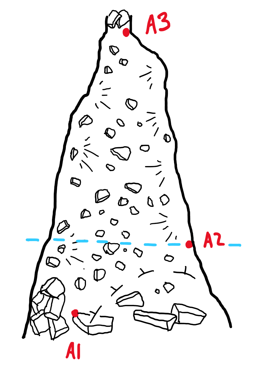
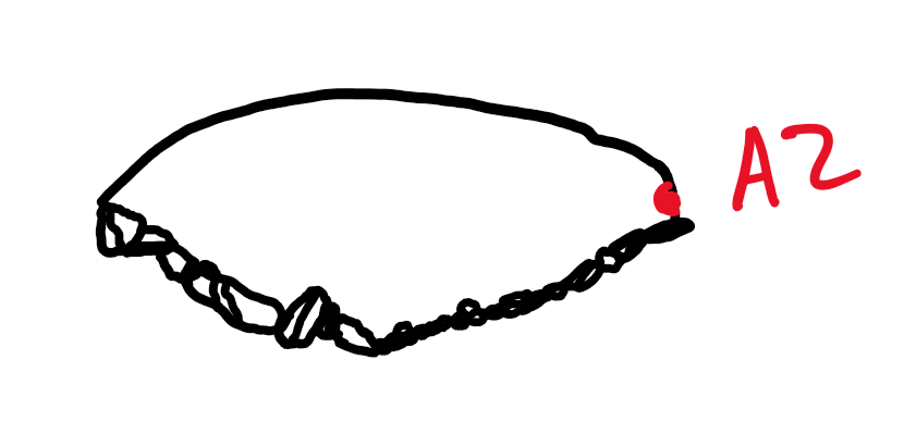
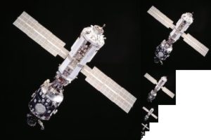
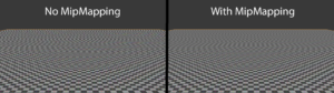
Mipmaps
Mipmaps create a hierarchical pyramid of textures as shown in the image above. Using mipmaps greatly reduces rendering artifacts by enabling the graphics card to sample the image properly. Some graphics cards (specifically older Intel integrated chips) do not implement DXT1 Compression and Mipmap correctly. As a result, CaveWhere may get black images instead of a useful cave map. To fix the black rendering, disable Mipmaps or Texture Compression. In this case, if you want the best quality, disable Texture Compression and enable Mipmaps. See below for an illustration of the difference between enabled and disabled Mipmaps in CaveWhere.
Mipmaps Enabled
Mipmaps Disabled
If you cannot tell the difference in the images above, here’s a more concrete example below.
Magnification Filter
Magnification Filter controls how OpenGL samples texture pixels when you view a texture up close. CaveWhere has two Magnification Filter options: Nearest and Linear. Nearest will render texture such that you can see individual pixels where Linear will blend them together. See the image below to see the differences. Magnification Filter is more of a visual preference than anything else.
Linear Magnification Filter. Check out how textures are blended together.
Nearest Magnification Filter. CaveWhere renders the images as pixels.
Minification Filter
Minification Filter controls how Mipmap layers are blended. When you zoom out, CaveWhere must blend mipmap layers together. CaveWhere supports four different Minification Filters: Anisotropy, Linear Mipmap Linear, Nearest Mipmap Linear and Linear. By default, CaveWhere uses Anisotropy filtering if your graphics card supports it. Anisotropy filtering gives the rendering the best quality.
If your graphics card does not support Anisotropy filtering, then you have to choose amongst Linear Mipmap Linear, Nearest Mipmap Linear, and Linear filtering. Linear Mipmap Linear is tri-linear filtering, Nearest Mipmap Linear is bi-linear filtering, and Linear is well Linear filtering. If you want to know the details, here’s Wikipedia to the rescue. Below shows the differences amongst all four filtering modes.
Linear Minification Filter
Nearest Linear Minification Filter
Linear Linear Minification Filter
Although CaveWhere detects your rendering settings automatically, sometimes it fails to detect the best texture filtering technique. If you are having rendering issues, like black textures, or textures fading in and out when you zoom, I recommend disabling Mipmaps or changing the Minification Filter to Linear, or possibility disabling Texture Compression.
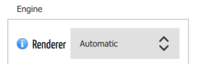
Engine Settings
To apply new Engine Settings, restart CaveWhere. The program supports three different renderers on Windows and two on MacOS and Linux. The first renderer, which is recommended, is OpenGL. If your system supports OpenGL renderer, it will give you the best support and best performance. Generally, when using Windows OpenGL renderer, graphics drivers have been installed.
If you have not installed your graphics drivers, CaveWhere will automatically fall back to OpenGL ES via DirectX. With OpenGL ES via DirectX, CaveWhere uses a graphics emulation layer called ANGLES to convert OpenGL ES to DirectX. This layer is only supported under Windows.
The final option is Software Renderer. The Software Renderer will always work but does not have DXT1 compression support and is by far the slowest renderer. The Software Renderer will use the CPU implementation of OpenGL and will never run on the graphics card. Software Rendering might be useful for running CaveWhere in a virtual machine. If CaveWhere crashes while checking OpenGL settings, by default it will fall back to Software Renderer.
Native Text Rendering
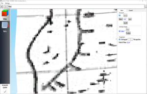
By default, CaveWhere uses Qt text rendering algorithm to render text in OpenGL and this option is disabled. Qt’s text rendering algorithm provides extremely fast and high quality text rendering. It’s recommended to keep this option disabled unless your computer is old and has a misbehaving graphics card. The image below shows an example of a misbehaving graphics card. If this happens, check the box to use Native Text Rendering. You can also try using OpenGL ES via DirectX to try to fix the artifacts.
Example of misbehaving graphics card rendering Qt texture rendering.
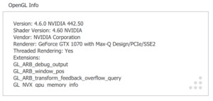
OpenGL Info
If you are ever curious what OpenGL version and extension that CaveWhere is using, OpenGL Info can help. Also, if you ever report a rendering issue, you can select and copy this information. It might help with debugging CaveWhere.